MIT 18.06 Lecture 1 — The Geometry of Linear Equations (Gilbert Strang)
Gilbert Strang opens MIT 18.06 by writing the same system of linear equations three ways — as rows (lines / planes meeting), as columns (linear combinations hitting a target), and as a single matrix equation Ax = b — and frames the course around the question of when that equation is solvable for every b.
Strang frames 18.06 as the start of n equations in n unknowns and tells students every lecture will read both a row picture and a column picture.
Title board: linear equations, n unknowns — [00:48]
Course is MIT 18.06 — linear algebra with Gilbert Strang.
Lecture 1 starts with n linear equations in n unknowns — the case where, generically, an answer exists.
Every problem in the course will be looked at both as rows (planes / lines intersecting) and as columns (linear combinations).
Goal of the hour: build the row picture, the column picture, and the matrix form for the same system, then ask when Ax = b is solvable.
Two equations, two unknowns — row picture
Strang writes 2x − y = 0 and −x + 2y = 3 on the board, plots the two lines on the (x, y) plane, and the unique solution falls out at their intersection.
2×2 example: matrix A = [[2,-1],[-1,2]] — [06:17]
System on the board: 2x − y = 0 and −x + 2y = 3.
Row picture: plot each equation as a line in the (x, y) plane.
The two lines cross at exactly one point — read off x = 1, y = 2 — and that pair solves both equations at once.
‘Row picture’ = look at one row of the system at a time and ask which (x, y) lies on that line.
Two equations — column picture and linear combinations
Same system, second viewpoint: each unknown is a coefficient on a column vector. The question becomes which combination of the two column vectors lands on b = (0, 3).
2×2 example: matrix A = [[2,-1],[-1,2]] — [06:17]
Rewrite the system as x · (2, −1) + y · (−1, 2) = (0, 3).
Column picture asks: what combination of the column vectors (2, −1) and (−1, 2) produces the right-hand side vector (0, 3)?
Reading the answer from the row picture (x = 1, y = 2), one copy of column 1 plus two copies of column 2 lands on (0, 3).
Strang stresses: column picture and row picture are the same problem in two languages — get used to reading both.
Three equations, three unknowns — row picture
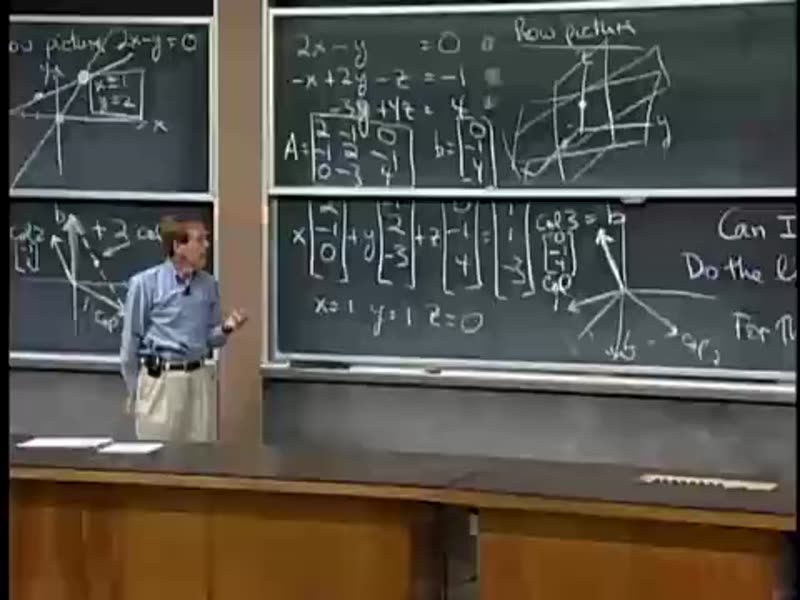
Bump the system up to 3×3 and the row picture becomes three planes in space; their common intersection is the solution.
‘N equations, N unknowns — row vs column picture, matrix’ — [14:15]
3×3 system on the board: 2x − y = 0; −x + 2y − z = −1; −3y + 4z = 4.
Row picture: each equation is a plane in (x, y, z) space.
Two planes meet in a line; a third plane usually cuts that line in a single point — the unique solution.
Row picture works in any dimension in principle, but it is hard to draw past 3D.
Three equations — column picture and 3-D combinations
Column picture in 3-D: ask whether the right-hand side b is a linear combination of the three column vectors. By construction here it is — Strang reads x = 0, y = 0, z = 1 right off the columns.
Column picture: 1·Col₁ + 2·Col₂ reaches vector b — [22:54]Synthesis board: both pictures + Ax = b + ‘Can I solve for every b?’ — [30:17]
Columns are (2, −1, 0), (−1, 2, −3) and (0, −1, 4); the right-hand side is b = (0, −1, 4).
Question becomes: which combination of the three columns produces b?
b is the third column itself — so the combination is 0·col₁ + 0·col₂ + 1·col₃, giving x = 0, y = 0, z = 1.
The column picture often makes the answer faster to spot when b is already one of the columns or an obvious combination.
Matrix form Ax = b and naming the players
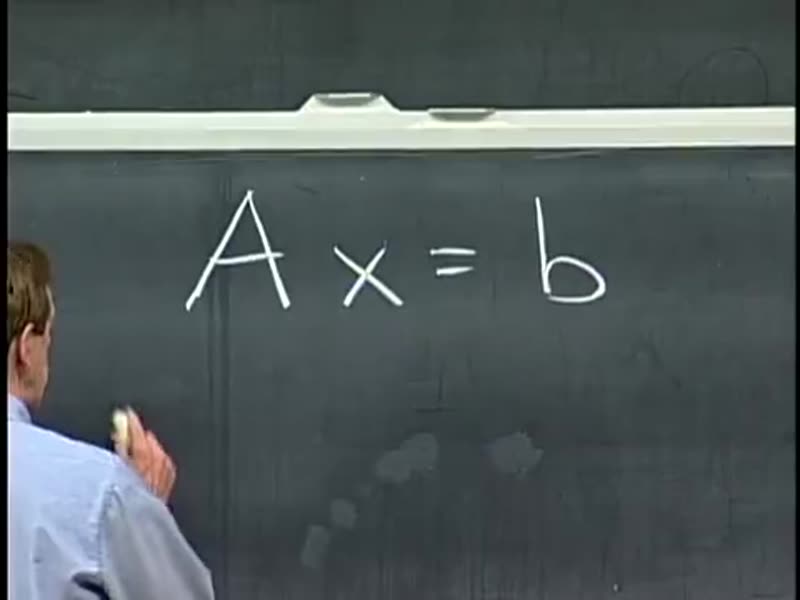
Strang packages the same system into Ax = b — A is the coefficient matrix, x the vector of unknowns, b the right-hand side — and points out that matrix-vector multiplication IS a linear combination of the columns of A.
Wrap-up: next time → elimination as a systematic method — [36:15]
Coefficient matrix A holds the columns; x is the unknown vector; b is the right-hand side.
Matrix-vector product Ax is literally x₁ · col₁ + x₂ · col₂ + … + xₙ · colₙ — a linear combination of A's columns weighted by the components of x.
Two ways to compute Ax: dot-product each row of A with x (row way), or take the combination of A's columns weighted by x (column way) — both must give the same answer.
Strang prefers the column way as the meaning of Ax = b for the rest of the course.
The big question: can we solve Ax = b for every b?
Closing arc: for which right-hand sides b is the system solvable? Geometrically — does the linear combination of A's columns cover all of n-space, or only a lower-dimensional piece of it?
Reframed problem: given A, can we hit every b in ℝⁿ as some combination of A's columns?
Yes precisely when the columns of A span ℝⁿ — equivalently, A is non-singular / invertible.
When the columns are linearly dependent the combinations only cover a plane (or line) in ℝⁿ — most b's are unreachable.
Hook for next lecture: elimination is the systematic way to find x when a solution exists, and to detect the singular case when it doesn't.
Key terms
row picture — 行图(按行看) Read each equation as one row of the system; in 2-D it is a line, in 3-D a plane; the solution is the point where all rows meet.
column picture — 列图(按列看) Read the system as a linear combination of the column vectors of A; the unknowns are the coefficients that hit the right-hand side b.
linear combination — 线性组合 A sum c₁·v₁ + c₂·v₂ + … of vectors with scalar weights — the construction underlying the column picture and the meaning of Ax.
coefficient matrix A — 系数矩阵 A The matrix whose columns are the column vectors of the system; writing Ax = b folds the equations into one compact statement.
right-hand side vector b — 右端向量 b The vector that the linear combination of A's columns must equal; in the row picture it sets where each plane meets the axis.
matrix–vector multiplication Ax — 矩阵–向量乘法 Ax Two equivalent definitions: dot each row of A with x, or take the combination of A's columns with weights x₁, x₂, …, xₙ.
singular matrix — 奇异矩阵 A square matrix whose columns are linearly dependent; its column combinations only cover a lower-dimensional piece of ℝⁿ, so most b are unreachable.
non-singular / invertible matrix — 非奇异 / 可逆矩阵 A square matrix whose columns span ℝⁿ — then Ax = b has a unique solution for every right-hand side b.
elimination — 消元法 The systematic procedure (introduced next lecture) for reducing Ax = b to a triangular system you can solve by back-substitution, and for detecting the singular case.

![2×2 example: matrix A = [[2,-1],[-1,2]]](frames/frame-02-377s.jpg)